CRBasic Tips to Simplify Data Post-Processing
de Barbra Utley | Atualizada: 08/12/2015 | Comentários: 3
Tópicos de blog
Area / Application


Product Category


Corporate / News
Pesquisar o Blog
Inscrever-se para o Blog
Receber e-mail quando um novo artigo é publicado. Escolha os temas de seu interesse.
Sugerir um artigo
Existe um tópico que você gostaria de saber mais à respeito? Nos informe.

You’ve collected your measurement data, but how do you easily make sense out of it? How can you simplify the post-processing of your data and start analyzing it sooner? In this article, I’ll explain how adding some code to your CRBasic program can save you from a post-processing headache later.
As a graduate student, I remember my colleagues often talking about the headache of post-processing data before they could even begin analyzing their data.
- For post-processing, some of us had learned how to write macros in Excel.
- Other colleagues preferred using resources such as Python, MATLAB, or R scripts to format their data for analysis.
- A group of us just slogged our way through, copying and pasting data into a new worksheet in Excel until all of the information was available in one spreadsheet—complete with extra columns of categorical labels.
As you might imagine, my colleagues and I found all of these post-processing methods to be cumbersome.
For our experiments in graduate school, we were encouraged to keep detailed notes on dates and times, as well as when an experiment moved from one treatment to the next. I understood the importance of keeping good notes, but I wondered if there was a way to save the information in the data table defined in CRBasic.
Most statistical software packages rely on data frames or input files that have a minimum number of columns and large quantities of rows or records. Too often, however, we format our raw data tables without considering the analysis we hope to complete after the data is collected.
Data tables typically include the default time stamp plus record number, and then we just start adding sensor measurements and system voltages. But normally, an experiment includes more—more treatments, more repetitions with multiples of the same sensor, just more information that is used to group the data for exploratory data analysis as well as T-tests, ANOVAs (analyses of variance), or regressions.
So, how can you store information like this in your data table for easy reference? I’ll step you through an example of how to create and manipulate categorical variables in CRBasic. The variables can be edited while the data is collected and stored in the data table.
Example
Note: Even if you’re not familiar with water quality and turbidity measurements, I think you’ll see in this example how easy it is to improve the helpfulness of your data table.
Background
In this example, the following question was posed: How does optical turbidity vary at six known concentrations (0, 10, 50, 100, 250, and 1000 mg/L)? To answer this question, data were collected using three OBS500 turbidity meters. The details of the experiment follow:
- Two hundred measurements were collected from each turbidity meter at each concentration.
- The measurements were collapsed into groups of 100 for mean, median, and standard deviation calculations.
- Different minerals were used to create sediment suspensions (quartz, kaolinite, bentonite, feldspar, mica, and coal). Natural river sediment was also collected, dried, sieved, and weighed to create natural sediment suspensions.
- The categorical variables included concentration (0, 10, 50, 100, 250, and 1000), sensor name (A, B, and C), and mineral (quartz, kaolinite, bentonite, feldspar, mica, coal, and natural sediment).
Original Data Table
The first round of data collection produced data tables similar to the one shown in Table 1. The reported values included the time stamp, record number, raw backscatter and sidescatter in millivolts, and backscatter and sidescatter readings in FBU (Formazin Backscatter Unit) and FTU (Formazin Turbidity Unit).
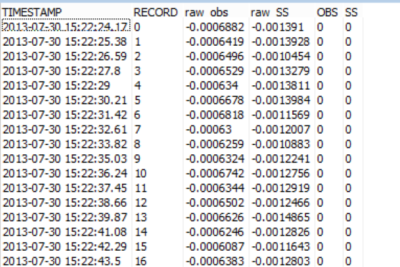
Table 1. Raw data collected during the sediment study.
For this experiment, the time stamp was not important because the measurements were not changing relative to time but to known treatments of sediment (concentration and mineral). Using the current data table setup in the CRBasic program running on my data logger, I had to rely on my detailed notes to post-process the data and figure out which sensor was used, what concentration was measured, and what mineral was used to create the suspension.
Improved Data Table
After making a few changes to the CRBasic program, I was able to generate a more detailed data table (Table 2) that includes categorical information defined as the following:
- obs500_meas(1) is backscatter (FBU).
- obs500_meas(2) is sidescatter (FTU).
- obs500_meas(5) is raw backscatter (mV).
- obs500_meas(6) is raw sidescatter (mV).
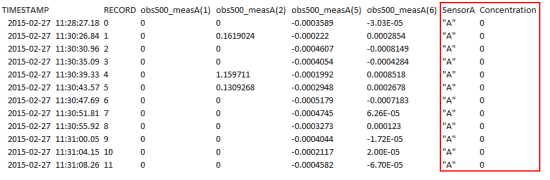
Table 2. Data collected for the natural sediment from sensor A at a concentration of 0 mg/L.
How to Do It
To transform my data table from Table 1 to Table 2, I only needed to add a few lines of code to the CRBasic program. Here’s how you can do it too:
- Define a few new variables for sensor and concentration. The sensor variables are defined as a 16-character string. The sensors are not public variables because they do not change. Concentration, however, is a public variable, so you can enter the known concentration into the public table.
Dim SensorA As String * 16

Dim SensorB As String * 16

Dim SensorC As String * 16

Public Concentration As Long
- Define the new data tables like this:
DataTable (SamplesA,1,10000)

	Sample (9,obs500_measA(),IEEE4)
	Sample (1,SensorA,String)
	Sample (1,Concentration,FP2)
EndTable


DataTable (SamplesB,1,10000)

	Sample (9,obs500_measB(),IEEE4)
	Sample (1,SensorB,String)
	Sample (1,Concentration,FP2)
EndTable


DataTable (SamplesC,1,10000)

	Sample (9,obs500_measC(),IEEE4)
	Sample (1,SensorC,String)
	Sample (1,Concentration,FP2)
EndTable
-
Define the sensor names within the program. Because we declared the sensors as “Dim” in our program, they will not show up in the public table. So, after your “BeginProg” statement, you will need to define the Name you want for each of the three sensors.
Tip: Remember that the sensors were defined as a 16-character-long string, so the name for each must be less than 16 characters.
In our example, A, B, and C were used. However, you could include serial numbers or model numbers of your sensors. These are not public variables in the sense that they are NOT changing with treatment. I collected 200 measurements per sensor in each treatment.BeginProg SensorA="A" SensorB="B" SensorC="C"
Now, every time a data table is called, the sensor string and concentration are added to the record as independent columns in the data table. It’s that easy!
Conclusion
I hope this example helps you understand how some simple additions to your CRBasic program code can save you from a post-processing headache later. Feel free to post your questions or comments below.


Sobre o autor
 Dr. Barbra Utley is a Project Manager at Campbell Scientific, Inc., working to support our global business processes. Previously, she was a Project Manager focusing on new-product introduction for the environmental market. She also was an Application Research Scientist in the Environmental Market Group. Barbra worked with both the Marketing and Engineering Departments on water resources product testing and development. Areas of interest include water quality and surrogate sediment measurements in freshwater systems, as well as statistical analysis. Barbra has a doctoral degree in Biological Systems Engineering with an emphasis in Water Resources.
Comentários
juanchit | 08/16/2017 at 12:48 PM
Hi Dr Barbra Utley.
We have 2 OBS501 Turbidimeters in our lab, and are deployig them both at the same time. As we don't use them at fix stations (but rather 1 minute stations at different locations), we have defined 3 Public Variables to i) open, ii) measure and iii) close the wiper from the PC400 software (we take the laptop to measure at all stations, just to check the instruments are measuring correctly).
But now we would like to add an extra variable in our table where we can store the name of the different stations, and we want to be able to set these names from the PC400, just as we can set the "open", "measure" and "close" variables.
Is there a way we can do that?
I send you the .cr8 file we are using upto now, just in case this provides more clarity.
Thanks a lot!
Juancho
'CR800 Series
'Created by Short Cut (3.0)
'Declare Variables and Units
Public BattV
Public PTemp_C
Public OBS500(4) 'direccion del sensor es O
Public OBS500_2(4) 'direccion del sensor es B
Public StationNames As String
Public open As Boolean
Public measure As Boolean
Public close As Boolean
Alias OBS500(1)=BS_I2016
Alias OBS500(2)=SS_I2016
Alias OBS500(3)=Temp_I2016
Alias OBS500(4)=WD_I2016
Alias OBS500_2(1)=BS_I2017
Alias OBS500_2(2)=SS_I2017
Alias OBS500_2(3)=Temp_I2017
Alias OBS500_2(4)=WD_I2017
Units BattV=Volts
Units PTemp_C=Deg C
Units BS_I2016=FBU
Units SS_I2016=FNU
Units Temp_I2016=Deg C
Units WD_I2016=unitless
Units BS_I2017=FBU
Units SS_I2017=FNU
Units Temp_I2017=Deg C
Units WD_I2017=unitless
'Define Data Tables
DataTable(OBSs_501,measure,-1)
Sample(1,BattV,FP2)
Sample(1,PTemp_C,FP2)
Sample(1,BS_I2016,FP2)
Sample(1,SS_I2016,FP2)
Sample(1,Temp_I2016,FP2)
Sample(1,WD_I2016,FP2)
Sample(1,BS_I2017,FP2)
Sample(1,SS_I2017,FP2)
Sample(1,Temp_I2017,FP2)
Sample(1,WD_I2017,FP2)
EndTable
'Main Program
BeginProg
'Main Scan
Scan(5,Sec,1,0)
'Default Datalogger Battery Voltage measurement 'BattV'
Battery(BattV)
'Default Wiring Panel Temperature measurement 'PTemp_C'
PanelTemp(PTemp_C,_60Hz)
If open Then
SDI12Recorder(OBS500_2(),1,"B","M3!",1,0)
SDI12Recorder(OBS500(),3,"O","M3!",1,0)
open = false
measure = false
close = false
EndIf
If close Then
SDI12Recorder(OBS500_2(),1,"B","M7!",1,0)
SDI12Recorder(OBS500(),3,"O","M7!",1,0)
open = false
measure = false
close = false
EndIf
If measure Then
'OBS500 Smart Turbidity Meter (SDI-12) measurements 'BS_I2016', 'SS_I2016', 'Temp_I2016', and 'WD_I2016'
SDI12Recorder(OBS500(),3,"O","M4!",1,0)
'OBS500 Smart Turbidity Meter (SDI-12) measurements 'BS_I2017', 'SS_I2017', 'Temp_I2017', and 'WD_I2017'
SDI12Recorder(OBS500_2(),1,"B","M4!",1,0)
EndIf
'Call Data Tables and Store Data
CallTable(OBSs_501)
NextScan
EndProg
BarbU | 08/23/2017 at 11:22 AM
Juancho,
I am sorry for my slow response, but excited you are using this approach. You are almost there in your code. You need to add a line to the data table definition telling the data table to grab the StationNames variable. See below.
'Define Data Tables
DataTable(OBSs_501,measure,-1)
Sample(1,BattV,FP2)
Sample(1,PTemp_C,FP2)
Sample (1,StationNames,String)
Sample(1,BS_I2016,FP2)
Sample(1,SS_I2016,FP2)
Sample(1,Temp_I2016,FP2)
Sample(1,WD_I2016,FP2)
Sample(1,BS_I2017,FP2)
Sample(1,SS_I2017,FP2)
Sample(1,Temp_I2017,FP2)
Sample(1,WD_I2017,FP2)
'EndTable
The default size for your string variable is 24 bytes. You can make this smaller inside the variable definition to optimize storage space. If your station names are long you can make this bigger but it will eat into the available data table storage memory.
You will store the site name every time your OBS501 data is written to the table.
I hope this helps and good luck with the turbidity monitoring.
Barb
juanchit | 09/11/2017 at 06:09 AM
Hi!
Sorry for my late response as well! I don't know why my user account didn't announce me your reply.
It was so easy! I though I had to make something special that would allow me to change table values from the PC400 software, but was not the case.
Thanks Barb!
Juancho
Please log in or register to comment.